How PHDwin Helped Avert a $100 Million Mistake
An oil & gas acquisition due diligence case study, with a one-year look-back. In 2025, Dwayne Stewart showed how a buy-side evaluation built in PHDwin V3 exposed sell-side forecasts that opened a gap of more than $100 million. In 2026, he graded his own forecasts against 15+ months of new production data and published the hits and the misses.

A Bad Deal You Win
In upstream oil and gas M&A, the only thing worse than a good deal you lose is a bad deal you win. That truism, from Dwayne Stewart, MBA, P.E., founder of Foundation Energy Advisors, anchors two PHDwin Week presentations that together make one of the most practical cautionary tales on acquisition due diligence we have published.
This guide combines both talks. It covers what went wrong in the sell-side forecasts, how Stewart caught it, how his forecasts held up a year later, and what every petroleum engineer, A&D professional, reserves auditor and E&P decision-maker should check before signing.
The only thing worse than a good deal you lose is a bad deal you win.
Dwayne Stewart, MBA, P.E. — Founder, Foundation Energy Advisors
Six Things Worth Carrying Into Your Next Data Room
B-Factors Move Everything
Small changes to a hyperbolic exponent swing reserves and PV10 dramatically. In the Haynesville case, slightly aggressive B-factors lifted Proved reserves by about 23% on average.
One Plot Is Not Enough
Rate versus Time hid the problems that Rate versus Cumulative and Rate versus Delta Time exposed.
Forecast The Secondary Ratios
In strong water drive and waterflood assets, total fluids and water-oil ratio tell you whether a miss is a reservoir problem or an operations problem.
Stale Type Curves Hide Losses
Type curves built on first-generation wells and never updated with infill results keep uneconomic locations on the books.
Aggregate Before You Trust
Sum Plots and Stack Plots expose inflated assumptions that a well-by-well review can miss.
Engineering Is Cheap
In Stewart’s words, good engineering is very cheap compared to a bad deal.
Sell-Side Forecast Versus Buy-Side Evaluation
| Item | Sell-side forecast | Foundation Energy Advisors (buy-side) |
|---|---|---|
| Cerdo 2H oil EUR — strong water drive, Gulf Coast Frio sand | ~225,000 bbl | ~140,000 bbl |
| Cochon 2H gas reserves — Haynesville Shale | 14 to 14.5 BCF | ~11 BCF |
| B-factor on Cochon 2H | 1.25 | 0.51 — fit to boundary dominated flow |
| Proved Undeveloped reserves, 300 Cochon PUDs | 6.3 TCF | 4.9 TCF |
| Nine-well Cochon EUR — 2026 look-back | ~180 BCF (~1.7 BCF per 1,000 ft) | 140+ BCF (~1.3 BCF per 1,000 ft) |
Swipe to compare →
Why Due Diligence Can Never Be An Afterthought
Buyers carry the risk in an upstream deal, and the paperwork says so. Teasers and CIMs routinely include language in which the seller and its advisor disclaim all liability and the recipient agrees to run its own independent evaluation. In Stewart’s layman’s translation: if the acquisition fails, you have no one to blame but yourself.
Incentives make that warning more pointed. Sell-side advisory shops are typically motivated to maximize the transaction price, and nearly all of them are paid on a contingent fee basis. In Stewart’s view, that means SEC and PRMS reserve definitions “rarely matter to marketers,” and sell-side forecasts can drift toward the optimistic.
Stewart’s firm sees the buy side of this every day. Over the 12 months before his 2026 talk, Foundation Energy Advisors screened more than 150 acquisition targets for E&P and oilfield service clients, from the Gulf of America to the Dakotas and from the Rockies to Appalachia. More than two dozen made it through full evaluation, and a handful of deals were signed or in final negotiations.
The industry is littered with E&P companies that a bad deal, or a string of them, bankrupted. Stewart is not arguing against buying. He acknowledges there are often intangible reasons a company wants or needs an asset. His point is that rigorous economic evaluation lets the C-suite see whether a deal is accretive or dilutive before the money moves.

Four Shortcuts That Cost Buyers Money
The 2025 talk opens with four themes for improving forecast integrity. Read as a cautionary tale, each one is a shortcut that looks efficient in a data room and gets expensive after closing.
Mindless Automation
Automation carries assumptions nobody disclosed — allocated data for wells sharing a tank battery or Lease ID, where only the provider has the algorithm. In the Illinois Basin, neither Illinois nor Indiana reports oil, gas or water volumes, so a buyer relies 100% on the seller.
Oversimplified Assumptions
Offshore, a 90% fixed / 10% variable expense split is common; onshore most people flip it. In a strong water drive asset, oil declines while total fluids hold, so lifting costs stay flat. Assume 90% variable and you understate opex, which overstates reserves.
The Wrong Technique
Life is more than curve fitting. Auto-generated curves always give an answer, “even if that answer has zero basis in reality.” B-factors of 1.5 or 2+ are standard auto-fit output, and big B-factors produce big reserves.
Looking For An Engineer Button
Boutique banks increasingly use non-engineers to estimate reserves and future net revenue. They cannot certify a forecast. Stewart quotes Red Adair: if you think it’s expensive to hire a professional, wait until you hire an amateur.
El Cerdo Feo And The Forecast That Didn’t Match History
An anonymized onshore Gulf Coast field producing from Frio sands under a strong water drive.
On a semilog Rate versus Time plot, the seller’s projection for the Cerdo 2H looked a little aggressive but not egregious. Stewart never looks at Rate versus Time alone. He pairs it with Rate versus Cumulative, which he calls a pseudo material balance plot, and the problem became obvious.
The historical data ran along a straight line on the log Rate versus Cum plot, indicating a B-factor of 1 — a harmonic decline. A forecast that should have continued that trend instead broke away from it. In Stewart’s words, the seller’s forecast was “extremely suspicious.”
In a high water cut reservoir, total fluids stay fairly constant over time. Once the water-oil ratio climbs above roughly 2 to 5, fractional flow dominates the decline. So Stewart forecast total fluids and WOR, and let PHDwin V3’s High Water Cut phase configuration reverse engineer the oil forecast.
What The Buy-Side Found
- Foundation’s forecast came to about 140,000 bbl EUR on the Cerdo 2H. The seller’s methodology projected about 225,000 bbl.
- The seller used a typical onshore 10% fixed / 90% variable opex split. With total fluids holding steady, opex does not fall away as oil declines. Correcting it reduced reserves and raised the economic limit.
- PUD, Probable and Possible type curves were all built on first-generation 2015–2016 wells and never updated with infill results.
- The 2021 and 2022 wells were sub-commercial — payout reached, but at less than 10% IRR. The 2023 and 2024 wells were completely uneconomic.
Gradual write-downs
Stewart connects this to the ethics talk David Clark of Marathon gave at PHDwin Week 2025 on gradual write-downs: a series of small revisions over many years that avoid one large write-down and keep unjustified reserves on the books. Updating the type curves made every location uneconomic at once. Stewart’s read was that the operator appeared to be taking slow, small write-downs while preparing to divest.

In a strong water drive, mother nature supplies energy. In a water flooded asset, humans supply the energy.
Dwayne Stewart, MBA, P.E. — Founder, Foundation Energy Advisors
Le Vilain Cochon And The “Slightly Aggressive” B-Factor
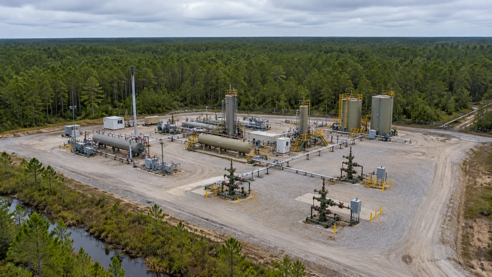
An anonymized Haynesville Shale dry gas field in Louisiana, with 300 PUD locations behind the producing wells.
For gas wells, Stewart adds a third plot: Rate versus Delta Time on a log-log scale. Delta Time is the number of days since the start of production, used as a proxy for Material Balance Time. A unit slope line marks a proxy for boundary dominated flow — the region controlling long-term reserves. Early data affected by choke management, linear flow or bi-linear flow gets excluded.
On the Cochon 2H, PHDwin V3 fit the boundary dominated flow region with a hyperbolic exponent of 0.51. That forecast came to a little over 11 BCF. The seller’s came to a little over 14 BCF — a gap of about 3 BCF on one well.
The seller’s B-factor was visible in the Default Projection Qualifier: 1.25. Anyone looking only at Rate versus Time would have missed it. “It would slip right through the cracks.” The seller had also tied its forecast to the last four months of data.
What It Was Worth
Across the field, slightly aggressive B-factors lifted Proved reserves by about 23% on average. On the 300 PUDs alone, that came to an aggregate difference of 1.4 TCF: Stewart’s team estimated 4.9 TCF of Proved Undeveloped reserves, the seller 6.3 TCF.
At 10 to 20 cents per MCF in the ground for proved dry gas, a 1.4 TCF overstatement translates to an overpayment on the order of $150 million to $300 million. The same pattern ran through the PDP wells and compounded on the PUDs.
The risk in arguing for a slightly more aggressive B-factor is that what you are calling Proved quietly becomes Probable, or even Possible.
What new production said
Stewart built the Cochon forecast with data through December 2024. By the time of his 2025 talk, about five more months of production had been loaded that morning. They followed his forecast, not the seller’s. Compared with the seller’s projection six months earlier, his forecast would have looked conservative. With more data, it was close to spot on.
The Cochon 9H was starker. Its Rate versus Cumulative curve bent concave down, which indicates a B-factor below 1, while the seller’s forecast bent concave up and did not honor the historical trend at all. On the Delta Time plot, production fell below the unit slope line, which pointed to a B-factor between 0 and 1. For Stewart, that was a red flag before any forecasting began: the seller’s B-factor was “not only wrong, it’s way too high.”
The Cochon 9H Was Starker
- Its Rate versus Cumulative curve bent concave down, indicating a B-factor below 1.
- The seller’s forecast bent concave up and did not honor the historical trend at all.
- On the Delta Time plot, production fell below the unit slope line, pointing to a B-factor between 0 and 1.
- A red flag before any forecasting began: the seller’s B-factor was “not only wrong, it’s way too high.”
What PHDwin V3 Made Visible
| Capability | What it let Stewart do |
|---|---|
| Rate-Time and Rate-Cum plots side by side | Read the likely B-factor before projecting. A straight line on semilog Rate-Time means B = 0 (exponential). A straight line on log Rate-Cum means B = 1 (harmonic). Concave down on Rate-Cum means B < 1; concave up means B > 1. In V2 these plots lived on separate tabs. |
| Rate vs Delta Time (log-log) | Use days since start of production as a proxy for Material Balance Time. The unit slope line marks boundary dominated flow; the half slope line marks an infinite-acting fracture. |
| One-click BDF fit | Select the unit slope region and click BDF. PHDwin fits that region, and the hyperbolic exponent can be stepped up or down to see which value honors the history. A tick on the curve shows where hyperbolic decline switches to terminal exponential. |
| Default Projection Qualifier | See which B-factor a seller used. On the Cochon 2H it showed 1.25. |
| High Water Cut phase configuration | Forecast total fluids and WOR, and let PHDwin build the oil and water forecasts from them. |
| Integrated reporting | Run economics and graphs together, without Crystal Reports or Batch Reports. Rate-Time, Rate-Cum and Delta Time graphs sit beside each well’s economics, with a hyperlinked Document Map. |
Grading The Forecasts Against 15+ Months Of New Production
The 2025 video went on to pass 11,000 views, and the PHDwin team asked Stewart to revisit both fields. His own framing: the video was about to make him, his forecasts and his firm look “really good or really bad. What could possibly go wrong?”
The setup was deliberately simple. He opened the previous year’s database, duplicated the scenario with a new report date of July 1, 2026, and copied last year’s forecast qualifiers into it with the Global Editor. He updated production only — no new lease operating statements, differentials or shrinkage. Last year’s projections were the starting point, and the new data were the test.

The Scorecard
| Well | Result against the 2025 forecast | What it meant |
|---|---|---|
| Cerdo 1H | On forecast. Total fluids and WOR on trend. | No change needed. |
| Cerdo 2H to 6H | Total fluids down by roughly 30% to 80%, so oil missed. WOR on trend. | An operational problem, not a geological one. |
| Cerdo 7H | Total fluids rising, oil roughly flat. | Rising fluids can mask decline. Expect a return to decline once they stabilize. |
| Cochon (most wells) | Production overlaying the prior forecast, well over a year past the December 2024 cutoff. | The boundary dominated flow forecasts held. |
| Cochon 1H | Erratic behavior after a shut-in. | Due a negative technical revision. |
| Cochon 4H | Overperforming after a shut-in. | Possible positive revision, but check operations first. |
| Cochon 9H | Underperforming its forecast. | Check for a pressure-system or choke change before revising. |
Cerdo Feo: The Water-Oil Ratio Told The Story
On the Cerdo 2H through 6H, oil production missed because total fluids fell sharply. In one well, total fluids dropped from roughly 20,000 barrels a month to about 3,000. But the water-oil ratio stayed on trend.
That is the point of forecasting secondary ratios. Had Stewart forecast oil alone, he would not know whether he was looking at a reservoir problem or a forecast problem. Because WOR held, the miss pointed to operations. The next step is a conversation with the operations team: can they restore total fluids? If yes, a negative technical revision is not yet warranted. If no, it absolutely is.
You do not want to project through a flat oil production with inclining Total Fluids. You’ll bust your forecast every time.
Cochon: Afterflow, Flush Production And The Temptation To Revise
- Shut-ins produce flush production. In micro-Darcy and nano-Darcy permeability, afterflow can last months or years, versus minutes or hours in high-perm conventional reservoirs. The Cochon 5H was back on its pre-shut-in forecast within one to three months.
- Check operations before you revise. An underperforming well may have been swung into a higher-pressure system during compressor maintenance or a flow line leak.
- Be honest about the misses. Stewart gave the Cochon 4H to the seller’s forecast for now, and called the Cochon 1H a clear miss for both.
- BDF assumes nothing changes. A choke change, a different operating system or a nearby offset well changes the drainage picture.
The Sum Plot: Where The Sell-Side Forecast Gave Itself Away
Individual wells over- and underperformed, but when Stewart summed all nine Cochon wells, the misses largely offset each other. That made the comparison with the seller stark. Excluding two months of downtime, actual production tracked Foundation’s forecast and sat well below the seller’s forecast from a year earlier.
The seller’s Sum Plot bent concave up, contradicting the concave-down behavior of the actual data. For what Stewart describes as a shallower, fringe asset that should come in under 1.5 BCF per 1,000 feet, the lower number is the one that fits.
The difference traces back to one step: identifying the unit slope on the Log Rate versus Delta Time chart, finding the boundary dominated flow regime, and curve fitting underneath it.

Three Lessons And The Pitfall That Goes With Each
Do Not Ignore Secondary Products
Gas-oil ratio, yield and water-oil ratio carry information. Ignore them “at your own peril.” They tell you whether a miss is a forecast problem, an operations problem or a reservoir problem.
Expect Flush Production
Resist a near-term positive revision after a shut-in. Most wells return to their prior forecast within 3 to 6 months. Step up reserves at year end because a well came back flush, and you will likely write the increase off.
Respect The Law Of Large Numbers
Granular forecasting is the industry norm, but Sum Plots and Stack Plots are the reservoir engineer’s best friend. Look for sharp inflection points at the effective date — production and forecast should join smoothly.
A Red-Flag Checklist For Sell-Side Forecasts
| Red flag in a seller’s forecast | What to check |
|---|---|
| The projection looks reasonable on Rate versus Time | View Rate-Time, Rate-Cum and Rate-Delta Time together. Look for a forecast that breaks away from the historical trend on Rate-Cum. |
| An aggressive B-factor the history does not support | Check the Default Projection Qualifier. Identify the unit slope region and fit it. Compare the forecast with the B-factor the data implies. |
| A forecast tied to only the last few months of data | Back the forecast up and see whether it would have predicted the earlier history. |
| Oil or gas forecast alone, with no secondary ratios | Forecast WOR, GOR or yield so you can separate reservoir behavior from operational changes. |
| A fixed and variable expense split chosen by geography | In strong water drive and waterflood assets, total fluids are nearly constant, so expenses are sticky. |
| PUD, Probable and Possible type curves from first-generation wells | Update them with infill results. Check parent-child interference and the returns on recent drilling. |
| A sharp change in slope at the effective date on Sum or Stack Plots | Aggregate the wells. A smooth join between history and forecast is the norm. |
| Production volumes you cannot verify | Ask how data was allocated, and check whether the state reports production at all. |
Frequently Asked Questions
What is a B-factor (hyperbolic exponent) in decline curve analysis?
The B-factor describes the shape of a decline curve. B = 0 is an exponential decline, B = 1 is harmonic, and a value between 0 and 1 is hyperbolic. Larger B-factors produce larger reserves, which is why they deserve scrutiny in due diligence. In PHDwin V3 you can estimate the likely value from plot shape: a straight line on semilog Rate-Time means 0, a straight line on log Rate-Cum means 1, concave down on log Rate-Cum means less than 1, and concave up means more than 1.
What is boundary dominated flow, and why does it matter for reserves?
In Stewart’s workflow, boundary dominated flow is the region of production that controls the long-term decline. On a log-log Rate versus Delta Time plot, the unit slope line is his proxy for it. Earlier data affected by choke management, linear flow or bi-linear flow is excluded from the fit. If the term bothers you for an unconventional well, he says you can read BDF as “Best Decline Fit.”
Why use Delta Time instead of Material Balance Time?
Material Balance Time is cumulative production divided by the instantaneous rate at that point in time. Reserve engineers rarely have the data to calculate it accurately, and gas is more complicated than oil. Delta Time, the number of days since the start of production, serves as a proxy. Stewart calls it a very good proxy, especially in low-compressibility systems such as high water cut oil systems.
Why forecast total fluids and water-oil ratio in a strong water drive or waterflood?
At high water-oil ratios, fractional flow dominates the decline. Forecasting total fluids and WOR versus cumulative oil lets PHDwin reverse engineer the oil forecast with high confidence. It also separates reservoir behavior from operations: if WOR stays on trend while oil misses, the cause is more likely a change in total fluids than a failed forecast.
When is a technical revision to reserves warranted?
A negative revision is warranted when operations cannot restore the total fluids a forecast depends on, or when a well behaves erratically after a shut-in. A positive revision needs more caution. First confirm the cause is not a pressure-system change, a choke change or flush production from a recent shut-in, since most wells return to their prior forecast in 3 to 6 months.
What are afterflow and flush production?
In tight gas and shale wells, a shut-in well keeps flowing into the fracture network and wellbore. In reservoirs with micro-Darcy and nano-Darcy permeability, afterflow can last months or years, versus minutes or hours in high-permeability conventional reservoirs. When the well is turned back on, that stored pressure produces a burst of flush production that depletes quickly.
How can a buyer spot an inflated sell-side forecast?
Compare the forecast with history on more than one plot, check the B-factor the seller used, look for a forecast built on only the most recent months, review type curves for stale analogs, and examine Sum and Stack Plots for sharp inflections at the effective date. The checklist above puts these steps in one place.
Both Talks Are Free To Watch
Start with the 2025 original for the two case studies, then watch the 2026 look-back to see how the forecasts held up.
How PHDwin Helped Avert a $100 Million Mistake | Dwayne Stewart, MBA, P.E. | Reserves, M&A, A&D
PHDwin Week 2025 · more than 11,000 views. Continuing education credit is available; the 2025 Ethics session must also be viewed to apply for the certificate.
- Stewart’s background and the “bad deal you win” truism
- Four themes for forecast integrity
- Rate-Time and Rate-Cum plots in tandem
- Forecasting a high water cut oil well
- Rate versus Delta Time as a proxy for Material Balance Time
- The seller’s 1.25 B-factor, and five new months of data
- Case summaries: the $100M+ gap and the 1.4 TCF overstatement
- Non-engineers, black boxes and “no engineer button”
$100 Million Mistake Case Study: One Year Later | Dwayne Stewart, MBA, P.E.
PHDwin Week 2026 · 3,300 views. Stewart revisits both fields against 15+ months of new production data.
- A year of A&D due diligence and why it matters
- High Water Cut phase configuration in PHDwin V3
- Setting up the database: scenarios and qualifiers
- El Cerdo Feo: grading the oil forecasts well by well
- Shut-ins, flush production and afterflow
- The scorecard: Cerdo Feo
- Sum Plots, unit slope and EUR per 1,000 ft
- Lessons learned and pitfalls to avoid
The Cheapest Time To Find An Aggressive B-Factor Is Before Signing
If your team is evaluating an acquisition, a divestiture or a year-end reserves update, start here.
- See PHDwin V3 in action. Learn more at phdwin.com, or get started free with a demo.
- Watch both talks. The 2025 case study first, then the 2026 look-back.
- Browse the full PHDwin Week lineup. The 2025 and 2026 sessions are on YouTube.
- Talk with the presenter. Connect with Dwayne Stewart and Foundation Energy Advisors, or contact PHDwin.
Sessions That Extend These Themes
The Perils Of The Black Box
Thad Toups, Haas & Cobb · PHDwin Week 2025 — auto-forecasting, B-factors and flow regimes.
Ethics In Engineering
David Clark, Marathon · PHDwin Week 2025 — gradual write-downs, referenced in Case 1.
Waterflooding: Enhancing Asset Value
Tad Fielder, Haas & Cobb · PHDwin Week 2026 — more on water-driven assets.
Dwayne Stewart, MBA, P.E.
Founder and Managing Member of Foundation Energy Advisors, a firm providing bespoke management, petroleum engineering and consulting services primarily in the upstream oil and gas sector.
Stewart began his career at Exxon in the mid-1990s, first in its cryogenic gas plant group and then in reservoir engineering. He joined Netherland, Sewell & Associates in 2004 and later served as Corporate Reserves Manager at BreitBurn. He has built upstream and midstream economic forecasts for three decades.