A Complete Field Guide to Rate-Time Analysis
Everything your reservoir team needs — from exponential to harmonic, nominal to effective.
6 slides covering every equation, key parameters, and PHDwin-specific implementation details.
Exponential
Constant percentage decline. Most conservative model.
Hyperbolic
Variable decline. Most common for real reservoir behavior.
Harmonic
Special case: b = 1. Gravity-drainage wells.
Effective
Readable directly from a production graph.
Cumulative Production Formulas
Integrate the rate equation to calculate EUR and recoverable volumes.
- PHDwin uses cumulative-volume differencing to minimize rounding errors over long forecasts
- Time does not need to be an integer — decimal months handle varying day counts automaticall
Exponential Cumulative
Np = (qi − q) / D
Hyperbolic Cumulative (b ≠ 1)
Np = qi^b / ((1 − b) · Di) · (qi^(1−b) − q^(1−b))
Harmonic Cumulative (b = 1)
Np = (qi / Di) · ln(qi / q)
Hyperbolic Rate Equation
The general form. Controls most real reservoir production behavior.
- Single porosity Good drive energy: b typically between 0 and 1. PHDwin default assumption.
- Fractured / dual porosity Poor drive or gravity drainage: b may range up to 2.0–2.5, rarely higher.
Rate Equation
q(t) = qi · (1 + b · Di · t)^(-1/b)
b
Hyperbolic exponent — controls curve concavity
Di
Initial nominal decline [Fraction / Unit Time]
Single Porosity
Good drive energy: b typically between 0 and 1 (Default assumption in most models)
Fractured / Dual Porosity
Poor drive or gravity drainage: b may range up to 2.0–2.5, rarely higher
Want to know more about equations?
Get in touch with our team of reservoir engineering experts to learn more about equations and how they can be applied to solve real-world challenges, optimize performance, and support better decision-making across your projects.
5 Rules PHDwin Gets Right
Implementation details that separate accurate forecasts from erroneous ones.
Follow for more technical education on decline curve analysis, EUR calculations, and reservoir engineering best practices.
01.
Curve fits always back up to the start of a month — no production lost from high early rates.
02.
Tangent effective decline only — eliminates confusion between Tangent and Secant methods.
03.
Decimal time (not integer months) is supported — day-count accuracy built in.
04.
Cumulative-volume differencing minimizes truncation and rounding error over long forecasts.
05.
Unit consistency enforced — D · t must be dimensionless, or results are meaningless.
Effective vs. Nominal Decline
Two ways to express decline — one intuitive, one for calculations.
Effective (Dₑ)
Read directly from a production graph. “Rate dropped X% this year”. PHDwin uses Tangent method as standard
Nominal (D)
Used inside equations. Cannot be read directly from a graph. Must be converted from Dₑ before use
Conversion (Exponential / Tangent Effective)
D = −ln(1 − Dₑ)
For Secant effective decline: D = Dₛ (direct substitution)
PHDwin standardizes on Tangent method to reduce industry confusion
Monthly Effective from Annual Effectibe
Dₑ,mo = 1 − (1 − Dₑ,yr)^(1/12)
Exponential Rate Equation
The simplest decline model — constant nominal decline rate over time.
- D is a fraction — always divide percentage by 100 before using.
- Annual D ÷ 12 = monthly nominal D. Valid only for nominal decline, not effective.
Rate Equation
q(t) = qi · e^(-D·t) This is the hyperbolic equation where b = 0.
q(t)
Instantaneous rate at time t [Vol / Unit Time]
qi
Initial instantaneous rate at time 0
D
Nominal decline [Fraction / Unit Time]
t
Time — units must match D and q